The Munger Dog

Charlie Munger is a business partner and longtime friend of Warren Buffett, and the source of the following illustration of a principle in behavioral economics known as gain/loss asymmetry. Consider the family dog peacefully at rest in a corner of the room. It might be possible to quantify its level of contentment or happiness by measuring heart rate, endorphin level, or simply tail wags per unit time, but let’s consider this to be the animal’s neutral state of happiness. Next, let’s produce a bone for this loyal companion and observe its response. The tail wags more frequently, it might run around a bit, or make some noise, but it’s fair to say that the dog is measurably happier now with the bone. Now, what will happen when we remove the bone from our happy dog? An overly simplistic model might tell us that the dog will return to its original, neutral state, but that would be unlikely. How then could this gain and loss, netting zero, result in the dog’s unhappiness?

As it happens, there have been numerous experiments and observations confirming that people (and house pets) tend to be more motivated to avoid a loss than to attain an equivalent gain. Put another way, our sensation of well-being (or “utility”) is not a symmetric function when it comes to gains and their equivalent losses. It might be more accurately described by the following graph.
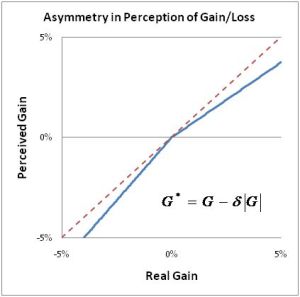
Asymmetry in Perception of Gain/Loss

Here, the perceived gain is discounted by an amount proportional to the real gain whenever the asymmetry parameter is positive.

Of course, this is a very simple model, so let’s also consider the effect that time might have on happiness. One can easily imagine that the dog’s happiness upon receipt of the bone will diminish with the passage of time. Let’s assume a simple accommodation model in the form of an exponential decay towards the neutral state, then our experiment might be described by the following graph.
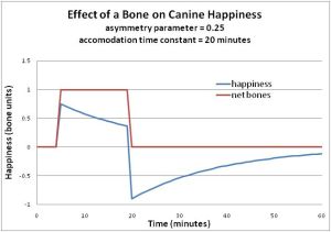
Effect of a Bone on Canine Happiness

Just for the pure heck of it, let’s write an equation for the model we’ve proposed:

Happiness Equation

Where H is “happiness”, B is “net bones” in possession, δ is the asymmetry parameter, τ is the accommodation time constant, and of course, t is time.

With such a model in mind, we can better understand the feelings and behavior of our companions (dogs and people have much in common), and even ourselves! I’m not saying that we need to actually solve the equation, or even assign quantities to the variables in order to benefit from the insight it offers (although it’s not really that difficult to solve). And that insight can be used in a variety of ways, from helping us devise an improved procedure for removing painful bandages, to explaining our trading behavior after we’ve had a good period of investment returns and then observe the inevitable “correction”.

Posted in Uncategorized | Tagged , , , | 2 Comments

How Far Is It to the Mall?

Some years ago as part of a family dinner conversation, one of my daughters asked a question … “How far is it to the mall?” It occurred to me that such a simple question could have many different answers.

First, we needed to establish which mall she had in mind. I preferred the Turfland Mall (it was closer, an easier drive, and less crowded) but after some discussion, it was clear that she was asking about the Fayette Mall. I suppose we could have just assumed she meant the closest mall that’s also “popular”.

Now having established a particular mall, what does she mean by “far”? A simple point-to-point distance (“as the crow flies”) is fairly unambiguous, but not particularly useful to most flightless 11 year-olds. Since she’s probably really interested in the distance along some surface route from our house to the mall, we need to establish a particular path along which to estimate the distance.

Selection of a route from our house to the mall will depend on whether you’re walking, riding a bicycle, or driving a car and so let’s now imagine we’re going to drive a car to the mall. Of the multiple reasonable routes, I suspect we would typically select a route based on perceived distance and anticipated traffic. This means that our route selection might be a function of the time of day, the season of the year, and who might be doing the driving. During rush hour, we could listen to the radio and include traffic reports in the decision-making process. There’s also a real possibility that we will change our route after we begin our trip based on traffic patterns or detours.

Notice that by assuming we want to avoid traffic, we’re actually making an assumption about the motivation for her asking the question in the first place. As we’re trying to restate her question in more precise terms, we’re assuming she might really be wondering how soon she can be at the mall (completely understandable given our typical dinner conversation). There’s even a chance that she might be interested in how much it will cost to get to the mall so we could discuss gas mileage (which is vehicle and route dependent), fuel prices, pro-rated insurance, car value depreciation, and other such things. Obviously, more information about her motivation in asking the question would help us tailor a more useful answer.

In any case, we’re dealing with some uncertainty here, and so a more complete and honest answer to her question would be to generate a graph and say something like: “We can’t know how long it will take to get to the mall but here is a distribution of likelihoods based on an assumed departure time and date.” And we could discuss methods for calculating these distributions of likelihoods well into our dessert.

I think somewhere during the course of the discussion, our daughter received the information she was looking for … and possibly a little extra. And while I don’t remember exactly how this particular discussion ended, I’m pretty sure no one was crying.

Posted in Uncategorized | Tagged , , , | 1 Comment

Sampling Bias and the Customer’s Perspective

On my 16th birthday I landed an entry-level position at Barney’s Drive-In, a small hamburger stand that (not coincidentally) employed a number of my friends from Purcell High School in Cincinnati. Barney’s was a relatively popular stop in Oakley Square in the years just before any of the chain fast-food restaurants located there. Having been to Barney’s as a customer, I knew it as a busy place with a line a customers waiting to be served.

Impressions change when your perspective changes, and after beginning work at Barney’s, I was surprised at the frequent, lengthy periods during which we had no customers in the store. How could it be that a place which seemed so busy before I was hired would seem comparatively desolate just afterward?

Without going into how either customer service efficiency or burger demand might have been affected by my presence, there is a simple explanation for my observation and it can also serve as an example of a type of sampling bias.

An employee’s impression of store crowdedness is based on observations that are uniformly distributed throughout the workday, while the customers’ observations are limited to those times when they are present. So let’s take a typical day and try to calculate the average number of customers in the store. The employee could set a timer and count people at specific intervals to get the data and the results might look like this:

sample time count count^2
1 10:00 0 0
2 10:30 1 1
3 11:00 3 9
4 11:30 5 25
5 12:00 15 225
6 12:30 12 144
7 13:00 6 36
8 13:30 1 1
9 14:00 0 0
10 14:30 0 0
11 15:00 0 0
12 15:30 2 4
13 16:00 0 0
14 16:30 5 25
15 17:00 8 64
16 17:30 3 9
17 18:00 9 81
18 18:30 8 64
19 19:00 5 25
20 19:30 7 49
21 20:00 5 25
22 20:30 0 0
23 21:00 3 9
24 21:30 0 0
25 22:00 2 4
total 100 800

In this example, 25 samples taken at uniform (and relatively arbitrary) times throughout the day and a total of 100 customers counted. From this data, the employee would conclude that the average number of customers in the store that day was 4.00. Now let’s try to survey the customers’ experience and ask each of them how busy the store was while they were there. This time we’ll get 100 responses and the one who showed up at 10:30 in the morning will say “1”, the 15 who were there at Noon will each say “15”, nobody’s there to say “0” for those several times when there’s no one there, and the two guys there at closing waiting for Rosie Sullivan to get off will say “2”. We’ll take this total (which is actually the sum of the squares of the previous observations) and divide it by the number of customers (100) to get a more “customer-oriented” average of 8.00. This is significantly higher (exactly twice in this admittedly contrived example) the more “employee-oriented” average.

So which average is correct? There’s not an easy answer to this question because it all depends on how you want to use the data! Besides that, a simple average generally can’t contain enough information about the distribution to be that useful. The important point is to understand here is that the customers’ perspective (if that’s important to you) is biased toward those occasions when more customers are present! Giving great service when you’re not busy doesn’t count nearly as much as giving great service when you are busy. And not understanding this could help you to achieve your goal of achieving perfect customer service … but in a perfectly empty store.

Posted in Uncategorized | Tagged , , , , | Leave a comment

Regression Analysis and the Importance of Knowing Something

My first “real” job after graduation was in the Mechanical Analysis department at IBM’s Office Products Division in Lexington, KY. We consulted with development engineering groups to help them with instrumentation, mathematical modeling, and general analysis. At that time (the late 1970’s), we often used APL (A Programming Language), an interactive, array-based programming language (and development environment) developed by IBM. It was remarkably advanced for its time and allowed engineers and scientists to quickly develop software to model systems or analyze problems without a lot of computer programming effort. Although APL is still available, it’s largely been replaced by applications such as MATLAB, Mathematica, Mathcad, and even Excel. A great thing about APL then (and about its successors today) was the abundance of well-written and useful software libraries (developed and shared internally among IBM’ers) and one of the more popular of the libraries used in our department was a workspace to perform regression analysis.

In regression analysis, data is analyzed to determine (or at least to hint at) the relationship between a set of independent variables and an observed response (the dependent variable). The concept fascinated me as I could design an experiment, run it, collect the data, enter it into an APL workspace, and then let the program tell me how the variables affect the observed response. There’s no apparent need for any fancy analysis or modeling, and regression analysis will at least tell you what direction you need to adjust each independent variable (“how to turn the knobs”) so that you can get closer to your desired output.

This is a rather simplified description of regression analysis, but the idea that it can be useful when you don’t know or understand the underlying nature of a system is quite seductive. This leads a lot of experienced engineers (and some of the instructors who informed my early understanding of regression) to underestimate the importance of developing a physically appropriate mathematical model of the system you seek to understand.

Most regression analysis software today allows you to choose from several model equations and options (linear, quadratic, multivariate, interactions, exponential, periodic, etc.). A fundamental understanding of the system under analysis can guide you to make the appropriate selections and the resulting regression model will better fit your data (better interpolation). More importantly, it will increase the predictive power of the model; in other words, the model will give more accurate results when the independent variables are outside of the range used to develop the model (better extrapolation).

In my experience, the proper regression equation is often not available using the software no matter how you might transform or combine the variables. In such cases, your best option is to derive an appropriate model equation and then perform the regression analysis “manually” … it’s not really that difficult. Generally try to use as few variables as possible (use dimensional analysis if possible). Calculate the residual error series as the difference between the predicted results (using the model equation) and the observed results (from the experiments). Then use an optimization routine to minimize the sum of the squares of these residual errors with respect to the parameters in your model equation. You will use the residual error sum of squares to estimate the significance of the regression terms.

What results from such an approach is not only a better and more predictive regression equation, but more importantly, a better understanding of the fundamental nature of the system. With a clearer understanding of your system, you will be able to think about the system more clearly, and this results in more efficient and inventive problem solving.

Posted in Uncategorized | Tagged , , , | 2 Comments